Introduction
Strain gauges produce signals that most measurement systems simply can't use directly. The resistance change in a loaded gauge—often a fraction of an ohm on a 120Ω or 350Ω base resistance—translates into a differential voltage output measured in millivolts or even microvolts. Feed that into a PLC, ADC, or data acquisition system without amplification, and you'll get noise, not data.
A strain gauge amplifier solves this. It provides stable excitation to the bridge, amplifies the tiny differential output by 100 to 1,000 times or more, filters out electrical noise, and delivers a usable analog or digital signal to downstream systems.
This guide gives engineers a working foundation for designing or selecting the right amplifier circuit — covering the Wheatstone bridge, instrumentation amplifier architecture, step-by-step circuit design, output configuration options, and real-world industrial applications.
Key Takeaways
- Strain gauge resistance changes are too small to process without amplification
- The Wheatstone bridge converts tiny resistance changes into a measurable differential voltage
- A strain gauge amplifier performs excitation, amplification, filtering, and signal conversion
- Resistor tolerance, gain setting, and reference voltage directly determine measurement accuracy
- Output type (analog voltage, current, or digital) must match the downstream data acquisition system
What Is a Strain Gauge? Understanding the Basics
A strain gauge is a resistive sensor—typically a thin foil grid bonded to a polymer carrier—whose electrical resistance changes proportionally when the material beneath it deforms under load. The challenge: that change is tiny. On a 120Ω gauge, strain from a structural load might shift resistance by a fraction of an ohm. Direct resistance measurement at that scale is impractical without specialized circuitry.
Why Constantan?
The conductive grid in most gauges is made from constantan, a copper-nickel alloy with electrical resistivity of 0.0000489 ohm-cm—roughly 29 times higher than copper's 0.00000170 ohm-cm. That high resistivity lets manufacturers pack a usable resistance value into a compact grid geometry. According to Vishay Micro-Measurements TN-505, constantan is the oldest and still the most widely used strain gauge alloy, with a gauge factor of approximately 2.0.
Gauge Types and Nominal Resistances
Two primary types are in common use:
- Bonded foil gauges: metallic foil grid laminated onto a flexible backing and adhered to the test surface; the standard for virtually all modern applications
- Wire-wound gauges: fine resistance wire formed into a grid; an older design still found in specialized or legacy applications
Standard nominal resistance values:
| Resistance | Typical Use | Key Trade-off |
|---|---|---|
| 120Ω | General-purpose measurement | Larger output signal; higher self-heating risk |
| 350Ω | Precision and long-duration tests | Reduced self-heating for a given excitation voltage |
| 1000Ω | High-accuracy transducer applications | Lowest self-heating; demands lower-noise amplification |
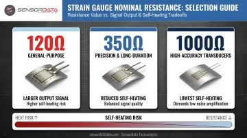
Nominal resistance selection shapes every downstream decision in amplifier design: excitation voltage, gain requirements, and achievable noise floor.
The Wheatstone Bridge: The Heart of Strain Gauge Measurement
A Wheatstone bridge is a four-resistor circuit where excitation voltage (Vex) is applied across two nodes and a differential output voltage is measured across the other two. When all four resistors are perfectly matched, the bridge balances and output voltage reads zero. Any resistance change—like strain deforming a gauge—creates a measurable imbalance.
Bridge Configurations
| Configuration | Active Gauges | Relative Sensitivity | Best For |
|---|---|---|---|
| Quarter-bridge | 1 | 1× | Structural monitoring, general testing |
| Half-bridge | 2 | 2× | Bending, axial compensation |
| Full-bridge | 4 | 4× | Load cells, torque sensors, high precision |
NI's strain gauge measurement data confirms this directly: quarter-bridge sensitivity is 0.5 mV/V at 1000 microstrain, while a full-bridge Type I reaches 2.0 mV/V—a 4× improvement. Full-bridge configurations also provide superior temperature compensation and common-mode noise rejection, which is why they dominate precision industrial applications like load cells and torque sensors.
The Output Voltage Formula
For a quarter-bridge under small strain conditions:
Vout = Vex × (ΔR / 4R)
With a 2.5V excitation voltage and a gauge factor of 2.0, the differential output at 1000 microstrain is just 1.25 mV. That number illustrates exactly why amplification is non-negotiable.
Excitation Voltage and Self-Heating
Excitation voltage sets both signal amplitude and self-heating. Higher Vex increases output but also increases power dissipation in the bridge resistors—causing thermal drift error.
There is no single universal excitation voltage. Per Vishay TN-502, the appropriate level depends on bridge resistance, gauge area, and the heat-sink capacity of the specimen.
The NI USB-9237 module illustrates this constraint well: it supports 2.5V to 10V excitation but caps total internal excitation power at 150 mW. Four 120Ω half-bridges are limited to 2.5V, while four 350Ω full bridges can run at 3.3V within that same budget.
The three fixed resistors in the bridge must precisely match the gauge's nominal resistance—use 0.1% tolerance or better. Mismatched resistors create a constant differential offset voltage that the amplifier amplifies right along with the signal, consuming output headroom before any load is applied.
With the bridge output characterized, the next challenge is conditioning that millivolt-level signal without introducing noise or gain error—which is where amplifier design takes over.
How a Strain Gauge Amplifier Works
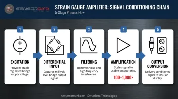
The amplifier isn't a single component—it's a signal conditioning chain with distinct stages:
- Excitation — A stable, regulated voltage drives the Wheatstone bridge
- Differential input — The millivolt-level bridge output feeds into the amplifier input
- Filtering — A low-pass filter removes high-frequency electrical noise
- Amplification — A gain stage boosts the signal by 100–1,000× into the usable range
- Output conversion — The conditioned signal is delivered as analog voltage, analog current, or digital data
The Instrumentation Amplifier Architecture
For strain gauge signals, the instrumentation amplifier (INA) is the preferred topology. It uses two input op-amps in a non-inverting configuration followed by a differential output stage, providing:
- Very high input impedance (the AD8221 specifies 100 GΩ ‖ 2 pF)
- High common-mode rejection ratio (CMRR)
- Single external resistor for gain setting
The AD8221 uses G = 1 + 49,400/RG and supports gains from 1 to 1,000. The TI INA333 uses G = 1 + 100,000/RG and achieves 100 dB CMRR at gains ≥ 100.
Those CMRR figures matter when compared against discrete alternatives. Analog Devices AN-589 shows that a unity-gain difference amplifier built with 1% resistors can have CMRR as low as 46 dB. Reaching 90 dB requires resistor matching to approximately 0.02%—a tolerance that's impractical in production. An integrated INA eliminates this problem by design.
Single-Supply Reference Voltage
Single-supply systems introduce a practical problem: without a negative rail, the amplifier can't represent compressive (negative) strain without clipping. The fix is to apply a mid-supply reference voltage (Vref = Vcc/2) to the INA's REF pin, shifting the output to mid-rail. TI's single-supply strain gauge reference design implements this with a precision voltage reference such as the REF5025, keeping the output centered and clipping-free across both tensile and compressive loads.
Filtering Trade-offs
Low-pass filters placed after amplification eliminate noise above the signal bandwidth of interest. The Micro-Measurements 2200 signal conditioner offers selectable four-pole Bessel low-pass filters at 1 Hz, 10 Hz, 100 Hz, 1 kHz, and 10 kHz—a practical illustration of the available range.
The core trade-off: lower cutoff frequency = better noise rejection, but slower response to rapidly changing loads. Quasi-static structural monitoring works well at 1–10 Hz, while dynamic fatigue testing or impact measurement requires 1 kHz or higher.
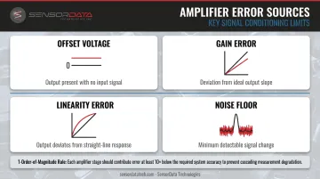
Key Error Sources
Every amplifier circuit introduces errors that must be managed:
- Offset voltage — output present with no load applied
- Gain error — deviation from the ideal output slope
- Linearity error — output deviates from a straight-line response across the full range
- Noise floor — minimum detectable signal change
A common design rule: amplifier errors should stay at least one order of magnitude below the sensor's own error budget. In practice, if your load cell specifies ±0.1% full-scale accuracy, the signal conditioner's combined offset, gain, and noise errors should fall below ±0.01% FS—otherwise the electronics become the weakest link in the measurement chain.
Strain Gauge Amplifier Circuit Design: Key Steps
Step 1 — Select and Match Bridge Resistors
R1, R2, and R3 must equal the strain gauge's nominal resistance (120Ω or 350Ω) and use 0.1% tolerance or better. Mismatched resistors create a constant offset the amplifier amplifies directly. That 0.1% figure is a practical floor: achieving very high CMRR may require tighter ratio matching or precision resistor networks.
Step 2 — Set Common-Mode Voltage and Bridge Current
A series resistor between the excitation supply and the bridge (often labeled R9 in reference designs) sets the common-mode voltage at the amplifier input to a value within the INA's input common-mode range. The value is calculated from:
R9 = (Vex − Vcm) / Ibridge
where Vcm is the desired common-mode voltage and Ibridge is the bridge current. Self-heating constrains maximum bridge current — thermal limits set an upper bound on excitation regardless of what the supply can deliver.
Step 3 — Calculate Required Gain
Gain = Desired output swing / Maximum differential input voltage
Worked example: A bridge produces ±2.25 mV differential input. Target output swing is 0.225V to 4.72V on a 5V single supply (leaving headroom at each rail). Required gain = (4.72 − 0.225) / (0.00225 × 2) ≈ 1,000 V/V.
For the AD8221: RG = 49,400 / (1,000 − 1) ≈ 49.4Ω
For the INA333: RG = 100,000 / (1,000 − 1) ≈ 100Ω
Step 4 — Verify Resistor Ratios for CMRR
With gain set, protecting it from common-mode interference becomes the next priority. In a two-op-amp INA, the ratio matching of external resistors (R1=R3, R2=R4) is critical: mismatched ratios degrade CMRR and cause the Vref voltage to appear at the output with gain other than 1 V/V, introducing a DC offset error. Select values from standard resistor series and hold 0.1% tolerance as the minimum.
Step 5 — Verify Linear Operation and Output Swing
Confirm that both the op-amp input common-mode voltage and output voltage remain within specified linear operating ranges across all strain conditions and supply tolerances.
For single-supply designs, follow these guidelines:
- Use rail-to-rail input/output op-amps to maximize usable output range
- Keep feedback resistor values low — high values degrade phase margin and add thermal noise
- Verify linearity across the full strain range, not just at nominal load
Types of Strain Gauge Amplifiers and Output Configurations
Output Types
Analog voltage (0–5V, ±10V)
- Direct connection to ADCs and PLCs with voltage inputs
- Preferred in low-power, short-cable, or legacy systems
- Simple wiring; susceptible to noise over long cable runs
Analog current (4–20 mA)
- Preferred in industrial environments with long cable runs
- Current signals are inherently noise-immune and self-monitoring (0 mA = wire fault)
- FUTEK ICA105 supports 0–20 mA, 4–20 mA, and other current output configurations
Digital (USB, SPI, UART, IO-Link)
- Integrates an onboard ADC; no separate signal conditioning needed
- USB variants (like FUTEK IDA100) allow direct PC connectivity
- IO-Link (IEC 61131-9) enables remote parameterization of gain, offset, filter settings, and alarm thresholds, making it well-suited for industrial automation environments where physical access is limited
- SPI-compatible ADCs such as the TI ADS1235 (24-bit delta-sigma) are purpose-built for bridge sensors and resistive pressure sensors
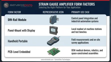
Form Factors
| Form Factor | Best Use Case |
|---|---|
| DIN-rail module | Control panel integration, industrial automation |
| Panel-mount with display | Local readout at machine or test station |
| Handheld portable | Field measurements, site surveys |
| PCB-level (embedded) | OEM applications: medical devices, robotics, space-constrained assemblies |
When selecting an amplifier, weigh these factors:
- Output type — voltage, current, or digital based on your system interface
- Bandwidth and ADC bit depth — match to required measurement resolution
- Supply voltage — verify compatibility with your power rail
- Environmental rating — IP65 minimum for harsh industrial environments
- Bridge resistance — confirm sensor compatibility before specifying signal conditioning
Industrial Applications of Strain Gauge Amplifiers
Strain gauge amplifier circuits appear across a wide range of demanding measurement applications:
- Load cells and weighing systems — Full-bridge configurations with high-gain INAs; standard in manufacturing process control and industrial weighing. All four bridge arms are active gauges, maximizing sensitivity and temperature compensation
- Structural health monitoring — Quarter-bridge or half-bridge arrangements on bridges, buildings, and aircraft structures where individual gauge placement is constrained by geometry
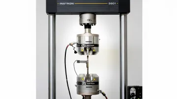
- Material and fatigue testing — High-bandwidth amplifiers (1 kHz+) required to capture dynamic loading events; sensors must endure millions of test cycles without drift
- Robotic force feedback — Compact PCB-level signal conditioners in precision assembly robots where space and weight are constrained
- Torque measurement — Full-bridge sensors on rotating shafts, requiring either slip ring or transformer-coupled signal conditioning
- Pressure monitoring — Full-bridge strain gauge-based pressure transducers in process industries
The global force sensor market was valued at USD 2.30 billion in 2024 and is forecast to reach USD 3.93 billion by 2035 at a 5.0% CAGR—a reflection of how broadly these measurement technologies have penetrated industrial systems.
That market growth is concentrated in exactly the applications where sensor design matters as much as the amplifier circuit: automotive component life testing, aerospace structural validation, and tire testing. SensorData Technologies, based in Shelby Township, Michigan, manufactures fatigue-rated load cells, torque transducers, and multi-axis sensors built specifically for these environments.
Their fatigue-rated load cells carry a formal guarantee against fatigue failure for 100 million fully reversed cycles, backed by AISI/SAE 4340 alloy steel construction. Product lines spanning pancake load cells, reaction torque sensors, and the fatigue-rated X-Y force sensor (Model M231, used in tire test machines) are built for high-cycle environments where amplifier circuit integrity and sensor longevity are both on the line.
Frequently Asked Questions
What is the purpose of a strain gauge?
A strain gauge measures mechanical deformation by converting dimensional changes into a proportional change in electrical resistance. That resistance change is processed by signal conditioning electronics to determine applied force, load, pressure, or torque.
What are the two types of strain gauges?
The two primary types are bonded foil strain gauges and wire-wound strain gauges. Bonded foil gauges—a thin metallic foil grid on a flexible backing adhered to the test surface—are the dominant type in modern use. Wire-wound gauges use fine resistance wire and are an older design, still found in some specialized or legacy applications.
What is the difference between 120Ω and 350Ω strain gauges?
350Ω gauges pass less current for a given excitation voltage, which reduces self-heating and thermal drift, making them preferred for precision and long-duration measurements. 120Ω gauges are more widely available and produce a larger raw output signal but are more susceptible to self-heating errors, particularly at higher excitation voltages.
What is a strain gauge amplifier?
A strain gauge amplifier (also called a signal conditioner) provides excitation voltage to the strain gauge bridge, amplifies the resulting millivolt-level differential output—typically by a gain factor of 100 to 1,000 or more—then converts it into a usable analog or digital output for data acquisition systems and PLCs.
What is a Wheatstone bridge and why is it used with strain gauges?
A Wheatstone bridge is a four-resistor circuit that converts the tiny resistance change of a strain gauge into a measurable differential voltage. It's used because direct resistance measurement of sub-ohm changes is impractical, but the bridge produces a voltage output that instrumentation amplifiers can accurately process.
What output types are available for strain gauge amplifiers?
Strain gauge amplifiers are available with analog voltage output (0–5V, ±10V), analog current output (4–20 mA for long industrial cable runs), and digital outputs including USB, SPI, UART, and IO-Link for direct integration with computers, PLCs, and Industry 4.0 networks.