Introduction
Sensors don't deliver measurement-ready signals on their own. A high-quality load cell or strain gauge produces a raw output that is weak, noisy, and often incompatible with the data acquisition system waiting to receive it.
Engineers working on automotive test rigs or fatigue testing frames know the frustration: the hardware looks right, the setup looks right, but the data doesn't behave.
The gap between sensor output and reliable measurement data is where signal conditioning does its work. It sits between the sensor and the DAQ system, and without it, even precision-engineered sensors deliver distorted results.
This article covers three specific, operational advantages signal conditioning provides — noise reduction, amplification, and linearization with calibration — and what happens when those functions are skipped or neglected. Each section addresses concrete outcomes: what changes in your data, and why those changes matter in high-stakes testing environments.
Key Takeaways
- Signal conditioning prepares raw sensor outputs — through filtering, amplification, isolation, and linearization — for accurate digitization.
- Ground-loop voltages of 10 mV or more can equal or exceed a load cell's entire full-scale output, making isolation essential to measurement accuracy.
- Without amplification, a 16-bit ADC may yield as few as 6 usable bits when reading a 10 mV bridge signal on a 10 V input range.
- Linearization and calibration are what convert a repeatable sensor into an accurate one — repeatability and accuracy are distinct, not interchangeable.
- Signal conditioning requires ongoing review, not a one-time setup.
What Is Signal Conditioning?
Signal conditioning is the set of operations applied to a raw sensor output before it reaches a measurement or control system. Those operations typically include amplification, filtering, isolation, excitation, and linearization — often several of these applied in combination depending on the sensor type and environment.
In the measurement chain, signal conditioning sits between the sensor (a load cell, strain gauge, force transducer, or torque sensor) and the DAQ system, instrument, or PLC that records or acts on the measurement. As the bridge between sensor and recorder, it determines whether the data at the output actually reflects what the sensor physically measured.
The Core Functions
| Function | What It Does |
|---|---|
| Amplification | Scales low-level sensor outputs to usable voltage ranges |
| Filtering | Removes electrical noise before it reaches the ADC |
| Isolation | Breaks ground loops; protects hardware from transients |
| Excitation | Supplies the reference voltage bridge-type sensors require |
| Linearization | Corrects nonlinear sensor response curves |
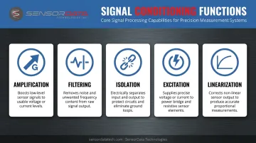
Each function addresses a different failure mode. Most real-world applications require more than one.
Key Advantages of Signal Conditioning for Measurement Accuracy
The three advantages below produce measurable, real-world outcomes: lower error rates, better data quality, and more reliable decisions.
Advantage 1: Noise Reduction for Cleaner, More Reliable Measurements
Industrial environments generate significant electrical noise. Motors, variable frequency drives, welding equipment, and power line interference all contaminate sensor signals — and the consequences aren't abstract.
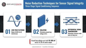
According to National Instruments, connected systems sharing the same building ground can differ in potential by 10 mV, 200 mV, or more. The problem: a common load cell produces a full-scale output of only 10 mV to 30 mV. A ground loop voltage can be the same order of magnitude as the signal itself.
How signal conditioning addresses this:
- Low-pass filters block high-frequency interference — including 50/60 Hz AC noise — before it reaches the ADC. The ADI AD7190, for example, provides 100 dB minimum rejection at 50/60 Hz at a 10 Hz output rate.
- Isolation breaks the ground loop path entirely, eliminating the periodic voltage error it introduces into the signal.
- Differential signal transmission attenuates common-mode noise across long cable runs.
Analog Devices describes ground-loop symptoms as drifting readings, measurement shifts when other equipment powers on, and a 60 Hz sine wave riding on top of what should be a DC measurement. None of those symptoms announce themselves as failures. They read as measurement noise or sensor instability — and get diagnosed as such.
When noise reduction matters most:
- Environments with heavy electrical machinery or VFDs
- Long sensor cable runs (50+ feet)
- Shared grounding between analog and digital circuits
- Sub-millivolt applications such as strain gauge or Wheatstone bridge measurements
KPIs affected: Signal-to-noise ratio, measurement error rate, system repeatability, false accept/reject rates, calibration drift frequency.
Advantage 2: Amplification for Improved Resolution and Sensitivity
Many precision sensors produce output signals that are far too weak for a DAQ system to digitize accurately. Strain gauges, load cells, and force transducers commonly output 1, 2, or 3 mV/V. With 10 V excitation, that is 10, 20, or 30 mV full scale — a fraction of the 0–10 V range most DAQ inputs expect.
The resolution consequence is direct and calculable. Using the ideal ADC code-span relationship, a 10 mV signal measured on a 10 V full-scale ADC range uses 1/1000 of the available input range. That represents a loss of approximately 9.97 bits of code span. A 16-bit converter effectively delivers around 6 usable bits across the signal; a 24-bit converter delivers approximately 14 bits — before accounting for noise or offset error.
Amplification closes that gap. Instrumentation amplifiers scale the signal (for example, from 0–10 mV to 0–10 V) while maintaining high common-mode rejection, ensuring the amplified output retains the fidelity of the original measurement.
Why this matters beyond resolution numbers:
In material testing or component life cycle validation, insufficient resolution means small structural changes or load variations go undetected. A test that should catch early-stage fatigue progression produces data that is simply too coarse to show it — not because the sensor missed the event, but because the amplification chain lacked the gain to make it visible to the ADC.
For sensors like SensorData Technologies' fatigue-rated load cells and force transducers — used in automotive powertrain testing and structural fatigue rigs — proper amplification is what makes the sensor's mechanical precision count at the data acquisition stage.
When amplification matters most:
- Low-output sensors: thermocouples, strain gauges, bridge-type transducers
- Long signal transmission distances where cable resistance degrades signal level
- Applications requiring detection of very small physical changes — micro-strain, fatigue cycle monitoring, medical force sensing
KPIs affected: Measurement resolution, ADC bit utilization, minimum detectable signal change, test repeatability.
Advantage 3: Linearization and Calibration for True Measurement Accuracy
A sensor can be perfectly repeatable and still systematically wrong. That distinction — between precision and accuracy — is exactly where linearization and calibration matter.
Many sensors do not produce an output directly proportional to the physical quantity being measured. The relationship between input and output follows a curve, not a line. Without correction, the system reports values that are internally consistent but wrong relative to reality. It will pass every repeatability check and fail every accuracy audit.
How linearization and calibration work:
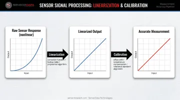
- Linearization converts the sensor's curved input-output response into a linear equivalent using a correction function derived from the known response curve. Implementation can be hardware-based (correction circuits) or digital (lookup tables or polynomial algorithms).
- Calibration then aligns that corrected output to a known reference standard, compensating for offset drift, temperature-induced variation, and manufacturing tolerances.
FUTEK specifies some load cells with nonlinearity, hysteresis, and nonrepeatability of ±0.02% of rated output. Interface defines nonlinearity as the maximum deviation from the ideal straight line, typically occurring around 40–60% of full scale and expressed as %FS. These are manufacturer-level values from precision sensors — in the field, without linearization and calibration, those deviations go uncorrected and accumulate.
The compliance dimension:
In regulated industries, measurement accuracy isn't a quality preference — it is a documented requirement. FDA 21 CFR 820.72 requires that inspection and test equipment be capable of producing valid results and that calibration procedures include accuracy limits and traceability to national standards. An FDA warning letter to Global Medical Technology cited failure to establish calibration procedures under 21 CFR 820.72(a) as a formal compliance finding.
ASTM E74-18, ISO 376:2011, and ISO/IEC 17025:2017 extend similar requirements to force calibration and testing laboratories. For aerospace, automotive, and defense applications, measurement traceability is a contractual and regulatory expectation, not an optional audit item.
When linearization and calibration matter most:
- Thermocouple-type sensors and Wheatstone bridge configurations
- Pressure sensors and transducers with known nonlinear response curves
- Applications where operating temperature ranges are wide or variable
- Regulated industries (medical, aerospace, defense, military)
Absolute measurement accuracy, calibration interval, compliance with ISO/ASTM standards, measurement traceability, and process yield rates all depend on getting linearization and calibration right — not just at commissioning, but across the sensor's service life.
What Happens When Signal Conditioning Is Missing or Ignored
Skipping signal conditioning doesn't produce an obvious system failure. It produces data that looks reasonable but isn't — and that gap between apparent and actual reliability is where the real operational risk lives.
The compounding failure modes:
Inconsistent results: Noise and signal instability inject random variation across test runs, making trend analysis unreliable and repeatability claims difficult to defend.
Undetected drift: Temperature-induced offset, ground loop interference, and ADC saturation accumulate silently — surfacing as audit findings or anomalous test conclusions rather than obvious errors.
Reactive troubleshooting: Engineers chase measurement anomalies that are symptoms of poor signal quality, not actual process events, driving up test time and labor costs.
Hardware damage: Voltage transients can damage DAQ hardware, sensors, and control electronics without isolation in place.
IEC immunity standards specify test levels of ±4 kV EFT on power lines and ±2 kV on signal lines — exposure levels that unprotected precision inputs aren't rated to handle. NI identifies improper grounding as one of the most frequent causes of DAQ damage, and the physics back that up: when ground loop voltages approach or exceed the full-scale signal range, every measurement downstream becomes suspect.
How to Get the Most Value from Signal Conditioning
Signal conditioning delivers results as a system-wide discipline — not a one-time hardware install. Its value depends on consistent application, periodic review, and alignment with the entire measurement chain as conditions evolve.
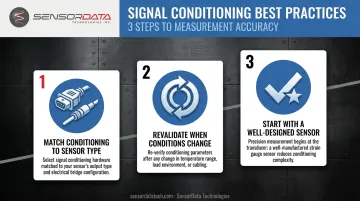
Three practices that maximize effectiveness:
Apply conditioning appropriate to each sensor type. Load cells, strain gauges, thermocouples, and RTDs each have distinct amplification requirements, linearization curves, and isolation demands — one unconditioned channel compromises the entire measurement chain.
Revalidate conditioning parameters when operating conditions change. New nearby electrical equipment, rerouted cables, or wider temperature swings can shift the noise profile the conditioner was originally configured to handle. Periodic checks — beyond initial setup — keep settings matched to real-world conditions.
Start with a well-designed sensor. Conditioning amplifies and cleans whatever the sensor provides — it cannot fix fundamental deficiencies in sensor construction. Sensors built to produce consistent, stable bridge outputs respond better to conditioning and yield more accurate end results. SensorData Technologies' fatigue-rated load cells and force transducers, for example, are engineered for this kind of stable, conditionable output across the full measurement chain.
Conclusion
Signal conditioning is the mechanism by which raw sensor output becomes measurement data worth acting on. In any application where decisions hinge on accurate readings — automotive testing, structural monitoring, medical device validation — the quality of that conditioning determines whether the data is trustworthy or merely plausible.
Noise reduction, amplification, linearization, and calibration each address a specific failure mode in the measurement chain. Together, they ensure that what the system reports reflects what is physically happening. Leave any one of them unaddressed, and you introduce a vulnerability that quietly erodes data integrity over time.
The discipline that produces reliable data is consistent: treat signal conditioning as an ongoing practice, not a one-time setup. Review it regularly, match it to the full measurement chain, and revisit it when environmental conditions or sensor configurations change. That's what separates measurement systems that inform decisions from ones that only appear to.
Frequently Asked Questions
What is meant by signal conditioning?
Signal conditioning is the process of preparing a raw analog sensor signal, through amplification, filtering, isolation, excitation, or linearization, so it can be accurately captured and interpreted by a digital measurement system or DAQ device. It occurs before digitization, in the analog domain.
What is the difference between signal conditioning and signal processing?
Signal conditioning happens before digitization, preparing the raw analog sensor output for accurate capture. Signal processing happens after digitization, manipulating the digital data mathematically.
What is signal conditioning in a PLC system?
In a PLC system, signal conditioning converts raw sensor outputs into standardized signal levels — such as 4–20 mA or 0–10 V — that the PLC's input modules can accurately read. It also provides isolation to protect the PLC from electrical noise and voltage spikes originating at the sensor end.
What are the main types of signal conditioning?
The primary types are amplification, filtering, isolation, linearization, excitation, and attenuation. Most real-world sensor applications require a combination of these, depending on the sensor type, output level, and electrical environment.
Why is signal conditioning especially important for load cells and strain gauges?
Load cells and strain gauges produce very small differential voltages (typically 10 to 30 mV full scale) that are highly susceptible to noise and far below standard DAQ input ranges. Instrumentation amplification, filtering, and isolation are essential to accurately digitize those signals before noise can distort the reading.
Can signal conditioning eliminate all measurement noise?
No. Signal conditioning significantly reduces noise, but achieving acceptable noise levels also requires proper grounding, shielded cabling, good PCB layout, and quality sensor selection. These work together. Conditioning alone cannot compensate for poor grounding or inadequate shielding in the installation.